My Data Is Dirty! Basic Spreadsheet Cleaning Functions

Tipsheet for Using Ocean Data in Your Investigations

No Coding Required: A Step-by-Step Guide to Scraping Websites With Data Miner

What Washington is Doing in Your Country: A Tipsheet for Investigating US Influence Around the World

Free, Game-Changing Data Extraction Tools that Require No Coding Skills
 In an extract from his new book Finding Stories with Spreadsheets, Paul Bradshaw explains how to use basic cleaning functions in spreadsheets to make it easier to combine data, including a case study where the same functions were used to speed up a research process for a story.
Whenever I’m working on a story involving combining data, it’s likely I will need to clean that data up in some way. Thankfully, Excel has a number of functions that take care of that repetitive work. We’ll cover many of these throughout the book, but we begin with the simplest: TRIM, CLEAN and SUBSTITUTE.
Those Pesky Spaces
The most basic is TRIM. This will trim extra spaces at the beginning and end of any cell. Spaces can be particularly problematic when working with data: you can’t see them, but the computer can. And if it’s trying to match two pieces of data – for example a region’s crime rate and the population for the same region – it will not match them if the region name has a space after it in one of the entries.
TRIM needs only one ingredient: the cell you want to trim spaces from. If you wanted to trim cell A2, then, you would write a formula like so:
=TRIM(A2)
The example above simply takes whatever is in A2, removes any spaces at the end and beginning, and puts it in the cell where you type the formula.
You can then copy this formula down the entire column to apply it to each cell in turn (A3, then A4, and so on), creating a new ‘trimmed’ or ‘cleaned’ column.
Find and Replace
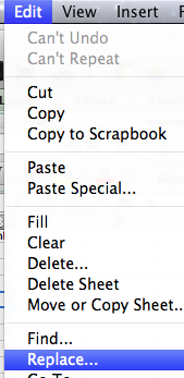 The Replace… option is in the Edit menu
Sometimes what looks like a space may actually be a slightly different character, which TRIM will not affect. In this case you may want to use the Replace… option in the Edit menu.
Before you select Replace… double-click on the cell containing the pesky non-space character and then click and drag to select only that character. Then copy it (the quickest way is CTRL+C or CMD+C on a Mac).
Once your Replace window is open paste it into the first box (Find what:). Leave the second box empty because you want to replace it with nothing. Click Replace all to see the results. It should also tell you how many replacements it’s made. That number should match the number of cells you think contain the character. If it’s higher it may have affected other cells as well.
If your problematic space is always in the same position (for example the first character) then you can also look into using the REPLACE function – dealt with in a later chapter.
Getting Rid of ‘Non-Printing’ Characters: CLEAN
The CLEAN function is designed to remove a number of invisible characters which are different to the basic space character and so cannot be dealt with by TRIM (although they will probably be dealt with individually by using find and replace as detailed above).
You can find a list of these characters at Ascii-code.com: they include things like carriage return, escape, back space and horizontal tab.
You use CLEAN just as you do TRIM: the function followed by a cell reference in parentheses like so:
=CLEAN(A2)
The result will be the contents of A2 minus any of those non printing characters.
You can of course combine both like so:
=CLEAN(TRIM(A2))
This uses the results of TRIM(A2) as the ingredient for the CLEAN function, so both are applied.
And or Ampersand? Substituting Particular Words or Characters
Spaces and non-printing characters are one thing, but what if you want to deal with other characters? That’s where SUBSTITUTE comes in. This is a cell-by-cell version of the Find and Replace option, which gives you much more control.
SUBSTITUTE needs three ingredients: the cell with the text you want to work with; what particular character or characters you want to substitute in that (if they are there); and what you want to replace that with.
There’s also a fourth, optional, ingredient: how many times you want to do the replacing.
SUBSTITUTE is particularly useful when you have one set of data which uses one convention, and a second which uses a different one, or a set of data which does not stick to the same convention at all.
For example, it’s quite common to find entries in a spreadsheet where an ampersand (‘&’) and the full word ‘and’ are used inconsistently, or two spreadsheets which use two different conventions. Others include:
- Percent vs %
- Decimal places to indicate thousands vs commas
- Dr vs Doctor vs no title at all
If we wanted to ‘clean’ some data to change the convention being used, we might use a formula like this:
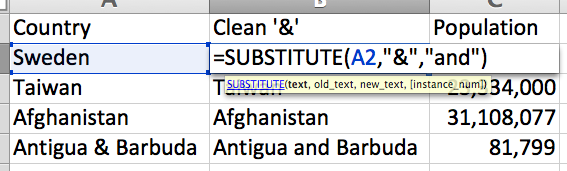
=SUBSTITUTE(A2,"&","and")
This means:
=SUBSTITUTE(THE CONTENTS OF A2, SUBSTITUTE '&', WITH 'AND')
If the cell does not contain the ‘&’ sign, then it is not substituted.
If for some reason, we only wanted it to substitute the first ampersand, we could use that extra argument like so:
=SUBSTITUTE(A2,"&","and",1)
But otherwise, it will assume we want to substitute all instances of ‘&’.
Again, when copied down a column, it will repeat this process on each cell next to it: A2 becomes A3, then A4, and so on.
Here’s an example of that in action with some country names – note that it makes no difference to names without an ampersand, but does change ‘Antigua & Barbuda’:
Replacing Something with Nothing
Of course you can use SUBSTITUTE to replace characters with nothing at all. Say, for instance, that we had a list of names but didn’t want titles complicating things, we could write the following:
=SUBSTITUTE(A2,"Mr","")
Or:
=SUBSTITUTE(A2,"Mrs","")
Both of these replace the two or three characters “Mr” or “Mrs” with “” – that is, nothing.
What if I want to substitute a quotation mark?
Because Excel uses quotation marks to indicate the beginning and end of a string of characters, it’s not easy to use quotation marks as just another character. For example, this formula, which tries to say ‘replace a quotation mark with nothing’ will generate an error: =SUBSTITUTE(A6,""","")
The solution is to use another function within Excel: CHAR. CHAR is used to convert codes used by computers into characters. These codes are called ASCII (American Standard Code for Information Interchange) and there are 255 numbers. For example, the letter ‘A’ is encoded as the number 65 by computers.
The ASCII code for quotation marks is 34. So instead of writing """, you can use CHAR(34). The formula in full using this would be=SUBSTITUTE(A6,CHAR(34),"")
Note that there are no quotation marks around CHAR(34) because this is not a string – it’s another formula. In fact, it’s what’s called a nested function, and we’ll deal with them in the next chapter.
Case Study: Generating URLs To Speed Up a Name Search

One investigation for the Mirror newspaper in the UK involved a spreadsheet containing hundreds of company names. In order to turn this into a story, we needed to identify the directors of each company, and then search to see if those individuals were connected with any newsworthy activity (for example, convicted criminals, political donors, tax evasion, subjects of frequent complaints, etc.)
The traditional method would see a person (or in this case, a team of journalism students) typing each company name into a website providing details on company directors, such as Duedil, or Companies House.
A repetitive process like this is a prime candidate for some computer assistance.
Rather than type in each name manually, then, we could use the =SUBSTITUTE function to help generate a URL for each company which would take the user directly to a page of search results.
Here’s what I mean:
A search for the company ‘Homezone Housing Ltd’ on Duedil generates the following URL:
https://www.duedil.com/beta/search/companies?name=Homezone%20Housing%20Ltd
A search for the company EBM Properties Ltd generates this URL:
https://www.duedil.com/beta/search/companies?name=EBM%20PROPERTIES%20LTD
Note that each URL is exactly the same apart for the name of the company at the end. In fact, we can express it like so:
"https://www.duedil.com/beta/search/companies?name=" followed by company name
If we have a series of cells containing company names the formula for adding each one to that URL would look like this:
="https://www.duedil.com/beta/search/companies?name="&A2
…where the company name is in cell A2 the first time.
When copied down, A2 changes to A3, A4, and so on.
But there’s one other thing about those URLs: any spaces were replaced in the browser with %20 – that’s because you cannot have spaces in a web address.
To add this extra bit of formatting, we can use the =SUBSTITUTE function to replace every space with %20. This can be done in a separate column with a formula like so:
=SUBSTITUTE(A2," ", "%20")
In other words: grab A2, but substitute every space, with the characters %20.
If this formula was in B2, we would then rewrite our SUBSTITUTE formula to grab the results like so:
="https://www.duedil.com/beta/search/companies?name="&B2
Of course you could skip that intermediate stage of substituting, and write a formula which combined both. That would look like this:
="https://www.duedil.com/beta/search/companies?name="&SUBSTITUTE(A2," ","%20")
All that this does is replace B2 with the formula we wrote in B2: =SUBSTITUTE(A2," ","%20")– but omits the = sign because that is only needed once, at the start of the formula (and we’ve already done that)
Note that you need to check the URL that is being generated first. For example, if you were sure that the companies were named accurately, you could skip the search results URL and jump straight to the company page URL instead. That looks like this – note that it uses dashes instead of %20 but also that you need a company number in part of the URL too (which you would also need in your spreadsheet):
https://www.duedil.com/company/IP28306R/homezone-housing-limited
Google uses the + sign, so your SUBSTITUTE formula would look like this:
=SUBSTITUTE(A2," ","+")
There’s also something else to consider: if your data has any extra spaces before or after the names, that will cause problems, so you may need to add the TRIM function, which gets rid of spaces at the start and end of cells. Again you could do this in a separate column like so:
=TRIM(A2)
…and then reference the cell with that formula in your next stage.
You could also combine both SUBSTITUTE and TRIM like so:
=SUBSTITUTE(TRIM(A2)," ","+")
The principle is, again, the same: you’re just replacing the cell reference with the formula that cell contains.
You could even combine all three stages like so:
="https://www.google.co.uk/search?q="&substitute(trim(A2)," ","+")
Recap
TRIMwill remove extra spaces before and after data in any cell. This is useful to ensure data is consistent and can be properly matched.- Some ‘special’ spaces are not affected by
TRIM, however, so if they’ve still not disappeared after usingTRIM, copy the offending space and use the Edit > Replace… option to paste that space character into the ‘find’ box, leaving the ‘replace’ box empty (so it is replaced with nothing). Make sure you note how many of these are replaced in your data (it will tell you) and that it matches what you would expect. SUBSTITUTEwill substitute a particular character (such as ‘&’) or string of characters (such as ‘and’) with whatever you specify (including no characters). This is similar to ‘find and replace’ but only affects the cell specified.SUBSTITUTEtakes three arguments: the cell containing the text you want to clean up; what you want to substitute (in quotation marks); and what you want to substitute it with.- If you only want to substitute the first, or the first two or three, instances of a particular character or string of characters, you can specify this in your formula as an extra argument after those.
- If no character/s is/are found, nothing is substituted.
- Because quotation marks are used to indicate a string, if you want to substitute a quotation mark itself you need to use another function:
CHAR. This is a way of indicating a character by its ASCII code. The formula to indicate a quotation mark, for example, is=CHAR(34)so using this within aSUBSTITUTEformula would look something like this:=SUBSTITUTE(A6,CHAR(34),"") - The
TRIMandSUBSTITUTEfunctions only work on one cell at a time, so copy them down an entire column to create a new ‘trimmed’ or ‘cleaned’ version of another.
 Paul Bradshaw runs the MA in Online Journalism at Birmingham City University, where he is an associate professor. He publishes the Online Journalism Blog, and is the founder of investigative journalism website HelpMeInvestigate.
Tipsheet for Using Ocean Data in Your Investigations
No Coding Required: A Step-by-Step Guide to Scraping Websites With Data Miner
What Washington is Doing in Your Country: A Tipsheet for Investigating US Influence Around the World
Free, Game-Changing Data Extraction Tools that Require No Coding Skills

This work is licensed under a Creative Commons Attribution-NoDerivatives 4.0 International License
Republish our articles for free, online or in print, under a Creative Commons license.
Republish this article
This work is licensed under a Creative Commons Attribution-NoDerivatives 4.0 International License
Read Next

Data Journalism News & Analysis
Lessons Learned: 10 Common Mistakes in Data Journalism
GIJN asked speakers and attendees in the NICAR conference hallways for the data journalism gaps they see, and for under-covered topic areas and under-used skills that newsrooms can address.

Data Journalism
10 Outstanding Data Projects Win the 2024 Sigma Awards
There were 52 data journalism entries from 22 countries in shortlist for the 2024 Sigma Awards. Here are the top 10 winning projects.
Tipsheet Data Journalism Reporting Tools & Tips
Tipsheet for Using Ocean Data in Your Investigations
Investigations into what happens on, under, and around the ocean can often be answered thanks to the vast amount of data available online.

Data Journalism Reporting Tools & Tips
Best Practices for Working With Mass Shootings Data
There can be confusion among journalists about “mass shootings” data, which leads to wildly different numbers and deeper confusion among audiences.